Basic geometric entities

Curve

Representations:

1. Explicit curve: $y = f(x)$

2. Implicit curve: $x^2 + y^2 = 1$

3. Parametrized curves: $\gamma(t) = (x(t), y(t))$

Modeling 1D Curves in 2D

Polylines

• Sequence of vertices connected by straight lines.

• Useful but not smooth.

Smooth Curves (Splines)

• Spline: Smooth curve determined by control points.

  • Interpolation: Passes through all control points.

  • Approximation: Does not pass through all points (more stable).

Bézier Curves

Definition:

Given control points $b_0, b_1, \dots, b_n$, the Bézier curve is:

$$b_n(t) = \sum_{i=0}^n \left(b_i \cdot B_i^n(t)\right), \ t \in [0,1]$$

where $B_i^n(t)$ is the Bernstein polynomial:

$$B_i^n(t) = \binom{n}{i} t^i (1-t)^{n-i}$$

Properties:

• Interpolates endpoints ($b(0) = b_0$, $b(1) = b_n$).

• Tangent to end segments.

• Affine transformation invariant.

• Convex hull property.

de Casteljau Algorithm:

Recursive linear interpolation to evaluate points on the curve.

Piecewise Bézier Curves

• Chain low-order Bézier curves for complex shapes.

• $C^0$ Continuity: Shared endpoint.

• $C^1$ Continuity: Shared endpoint + tangent continuity.

  $$a_n = b_0 = \frac{1}{2}(a_{n-1} + b_1)$$

General Spline Formulation

Definition:

A general spline can be expressed as:

$$Q(t) = GBT(t)$$

where:

• Geometry ($G$): Matrix of control points $(b_0, b_1, \dots, b_n)$.

• Spline Basis ($B$): Defines the type of spline (e.g., Bernstein for Bézier).

• Power Basis ($T(t)$): Monomials $(1, t, t^2, \dots, t^n)$.

Different spline types vary in their basis matrix $B$.

Surfaces

Parametrized Surface

Mapping $f: U \subset \mathbb{R}^2 \to \mathbb{R}^n$.

Example (Saddle):

$$f(u,v) = \begin{bmatrix} u \\ v \\ u^2 - v^2 \end{bmatrix}, \ \text{where } u^2 + v^2 \leq 1$$

Bézier Surfaces

Extend Bézier curves to 2D using control grids.

$$s(u, v) = \sum_{i=0}^n \sum_{j=0}^m p_{i,j} B_i^n(u) B_j^m(v), \ (u,v) \in [0,1]^2$$

Evaluation:

• Apply de Casteljau algorithm separately for $u$ and $v$.

Explicit Geometric Representations

Taxonomy

• Origin-dependent: Scanned data, procedural modeling.

• Application-dependent: Storage, rendering, animation.

Multiview 3D

• No explicit 3D geometry; reconstruction required.

Depth Maps

• Incomplete 3D; requires camera info.

Volumetric

• Voxel grids; high memory/computation cost.

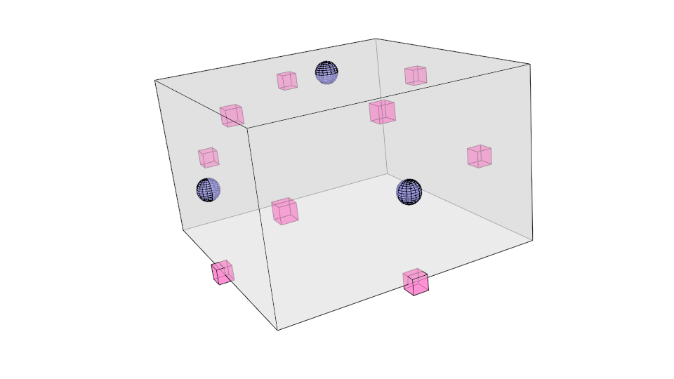
Point Clouds

• Unordered set of $(x,y,z)$ coordinates ($\pm$normals).

• Acquisition:

  • 3D scanning (LIDAR, Kinect).

  • Challenges: Noise, occlusion, registration.

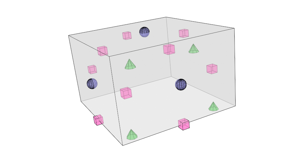
• Sampling Methods:

  • Uniform (i.i.d.).

  • Farthest Point Sampling (better coverage).

Polygonal Meshes

Triangle Meshes: Most common (simple, planar faces).

• $V = \{v_1, v_2, \dots, v_n\} \subset \mathbb{R}^3$

• $E = \{e_1, e_2, \dots, e_k\} \subset V \times V$

• $F = \{f_1, f_2, \dots, f_m\} \subset V \times V \times V$

• Manifold conditions

  • Each edge is incident to one or two faces

  • Faces incident to a vertex form a closed or open fan

What Should Be Stored?

• Geometry

  • 3D coordinates.

• Topology

  • Connectivity information between vertices, edges, and faces.

• Attributes

  • Normals, colors, texture coordinates.

  • Per vertex, per face, or per edge.

Data Structures:

• Triangle List (STL format).

  • Storage

    • Face: 3 positions

  • No connectivity information

• Indexed Face Set (OBJ, OFF formats).

  • Storage

    • Vertex: position

    • Face: vertex indices

    • Convention is to save vertices in counter-clockwise order for normal computation

  • Shared vertices

Mesh Processing:

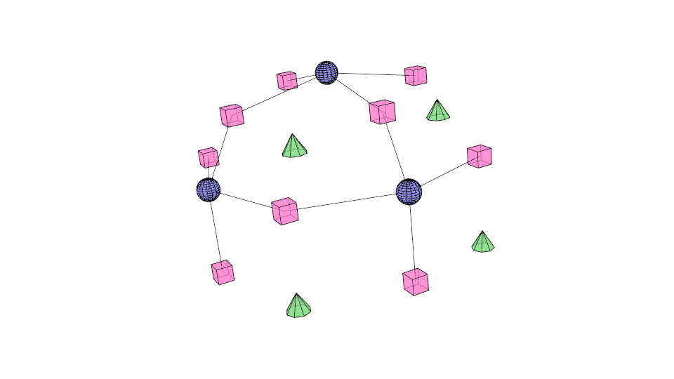
Mesh reconstruction

• Input: point cloud

• Output: triangle mesh

• Explicit Method

  • Hyper-parameter $\rho$

  • Assume a ball of radius $\rho$ cannot pass through the surface without touching the points.

  • Three points form a triangle if a ball of radius $\rho$ touches them without containing any other points.

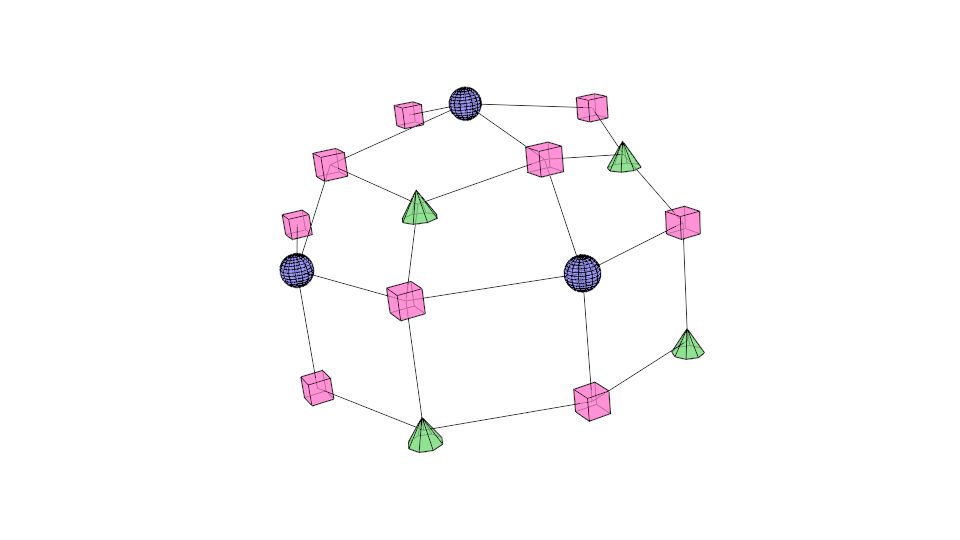
• Implicit Method

  1. Estimate an implicit field function from data

  2. Extract the zero iso-surface

Watertight manifold surface generation

• Many downstream tasks require this

• Meshes designed by artists or reconstructed by some algorithms often:

  • open boundaries

  • self-intersections

  • incorrect connectivity

  • ambiguous face orientations

  • double surfaces

• Huang J, Su H, Guibas L. “Robust watertight manifold surface generation method for ShapeNet models.”

  • Small artifacts, all surface have volume (https://github.com/hjwdzh/Manifold)

• Huang J, Zhou Y, Guibas L. “ManifoldPlus: A Robust and Scalable Watertight Manifold Surface Generation Method for Triangle Soups.” (https://github.com/hjwdzh/ManifoldPlus)

  • Less artifacts, may contain zero-volume structures

• Basic steps:

  • Voxelize the surface

  • Extracts exterior faces between occupied voxels and empty voxels

  • Projection-based optimization

Mesh subdivision (upsampling)

• Recursive upsampling

  • Divide mesh element

  • Calculate new positions of the mesh vertices

• Loop Subdivision

  • Split each triangle into four

    

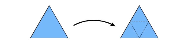
  • Assign new vertex positions according to weights

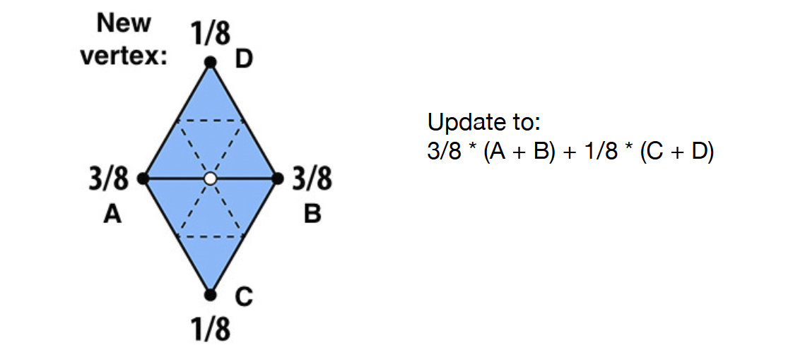
    • For new vertices

      

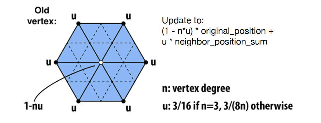
    • For old vertices

      

• Catmull-Clark Subdivision

  • Add a vertex (face point) in each face

    $$f = \frac{1}{n} \sum_{i=1}^n v_i$$

    

  • Add a vertex (edge point) for each edge

    $$e = \frac{1}{4}(v_1 + v_2 + f_1 + f_2)$$

    $f_1, f_2$ are the face points of the two faces sharing this edge

    $v_1, v_2$ are the two vertices of this edge

    

  • Update each old vertex

    $$v = \frac{f + 2m + (n-3)p}{n}$$

    $p$ is the old vertex position

    $f$ is the average of face points of faces adjacent to this vertex

    $m$ is the average of midpoints of edges incident to this vertex

    $n$ is the valence (degree) of this vertex

    

  • Form new edges and faces

    • Connect each new face point to the new edge points of all original edges defining the original face

      

    • Connect each new vertex point to the new edge points of all original edges incident on the original vertex

      

    • Define new faces as enclosed by edges

      

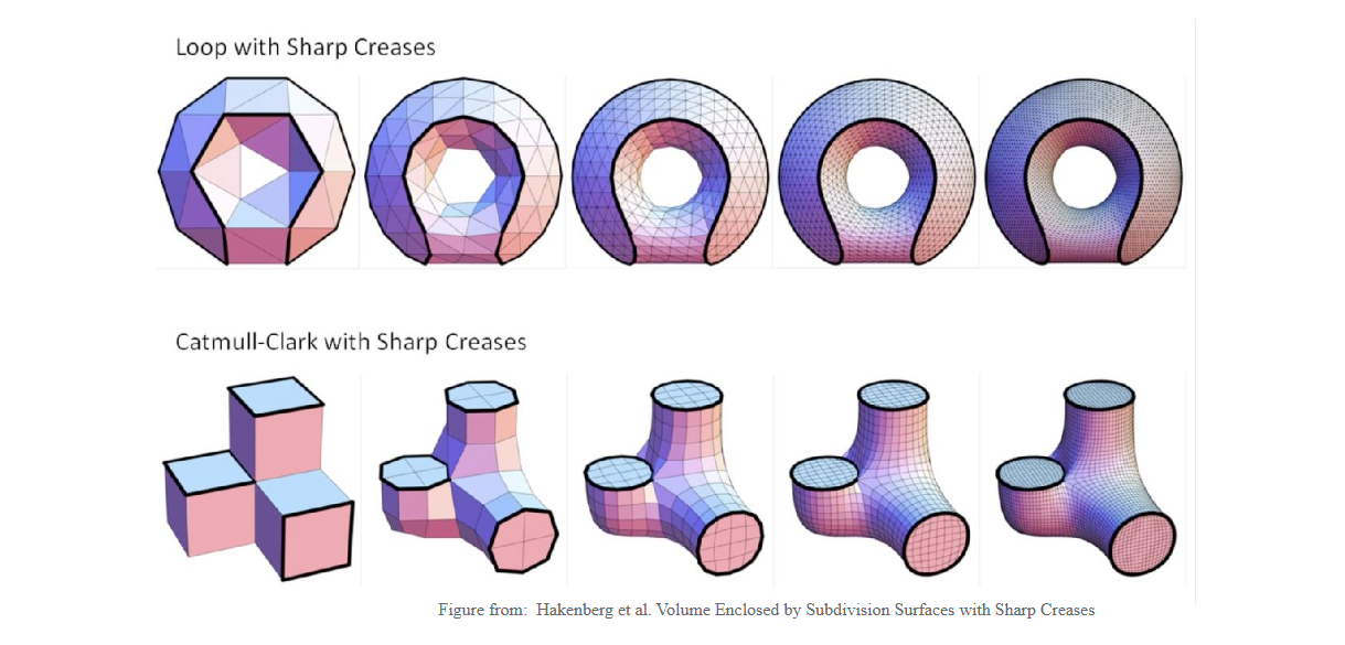
• Shape with Creases

  

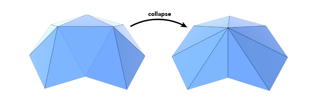
Mesh simplification (downsampling)

• Simplify a mesh using edge collapsing

  

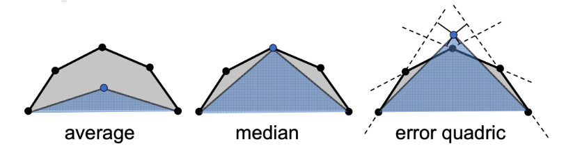
• Quadric Error Metrics

  Choose point $p$ to minimize the sum of squared distances to the planes of the triangles adjacent to the edge being collapsed.

  $$\min_p \sum_i \text{dist}(q_i, p)^2$$

  where the set of $q_i$ is all the faces incident to the two endpoints of the original edge.

  

• Which edge to collapse?

  • Assign score with quadric error metric

  • Use a priority queue to greedily collapse the edge with the lowest score

Mesh deformation

• Generate new meshes by deforming an existing one

• Use deformation energy

  • Translation and rotation should not change the deformation energy.

    

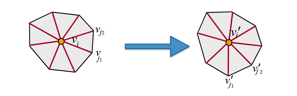
  • Stretching (length change) and bending (angle change) increase deformation energy.

    

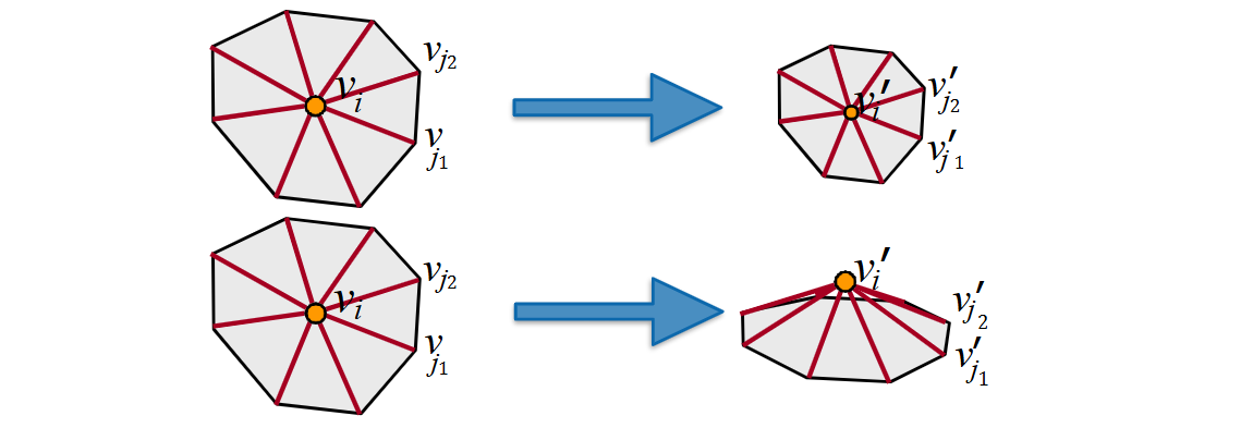
  • Local Deformation Energy (at vertex $i$)

    $$E(v_i) = \min_{R_i} \sum_{j \in N(i)} ||(v_i' - v_j') - R_i(v_i - v_j)||^2$$

    where $v_i'$ is the new position of vertex $i$, $v_i$ is the original position, $N(i)$ is the set of neighboring vertices of vertex $i$, $R_i$ is a rotation matrix (shared by cell).

  • Global Deformation Energy

    $$E(V') = \min_{V'} \sum_i E(v_i)$$

    where $V'$ is the set of all new vertex positions s.t.

    $$v_j' = c_j, \quad \forall j\in C$$

    where $C$ is the set of constrained vertices (e.g., dragged by user).

  • Minimizing total deformation energy

    • As-Rigid-As-Possible (ARAP) deformation

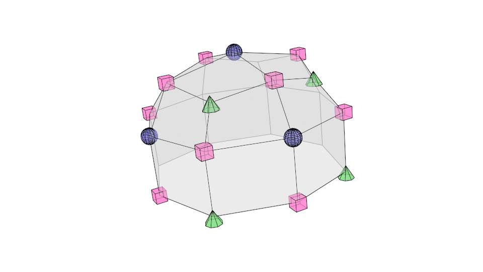
• 3D Free-Form Deformation (FFD)

  • Control points: 3D lattice

  • Modelers drag the vertices of the lattice to define displacements $\vec{d_i}$

  • Displacements of points in space are computed by interpolating $\vec{d_i}$ with interpolating weights $B_i$

    $$\vec{d}(x, y, z) = \sum_i \sum_j \sum_k B_i(x) B_j(y) B_k(z) \vec{d}_{i,j,k}$$

Implicit Geometric Representations

Definition: Surface = points where $f(x,y,z) = 0$.

Advantages:

• Easy inside/outside tests.

• Boolean operations (CSG)(construct solid geometry).

Challenges:

• Hard to sample points on surface.

Types:

• Algebraic Surfaces

  • Polynomial equations (e.g., spheres).

• Distance Functions

  • Giving minimum distance (could be signed distance) from anywhere to object

  • Instead of booleans, gradually blend surfaces together using distance functions

• Level Sets

  • Closed-form equations are hard to describe complex shapes

  • store a grid of values approximating function